FEniCS Solver Framework for VirtualCity@Chalmers

Introduction

During the past week we got done with implementing the basics for a solver framework. The solvers are written in the FEniCS¹-Python interface. So what do we mean by a solver? A solver is a function that returns an approximative solution to a partial differential equation (PDE) problem defined by given input data, i.e., problem data for the PDE such as domain and boundary conditions. At the moment there are two available solvers, one for solving the Stokes equations² and one for solving the advection-diffusion equation³. The two equations are presented below.

Stokes equations

The Stokes equations read: For a domain \( \Omega \subset \mathbb{R}^d \), where \(d = 2\) or \(3\), with boundary \( \partial \Omega \), find the velocity \( \mathbf{u} : \Omega \to \mathbb{R}^d \) and the pressure \( p: \Omega \to \mathbb{R} \) such that:

\begin{equation}
\left\{
\begin{split}
– \Delta \mathbf{u} + \nabla p & = \mathbf{f} && \ \text{in} \ \Omega, \\
\nabla \cdot \mathbf{u} & = 0 && \ \text{in} \ \Omega, \\
\mathbf{u} & = \mathbf{u}_b && \ \text{on} \ \partial\Omega,
\end{split}
\right.
\end{equation}

where \( \mathbf{f} \) is a given source term, and \( \mathbf{u}_b \) is given boundary value(s), e.g., inflow velocity and/or value \(\mathbf{0}\) for no-slip condition.

Advection-diffusion equation

The advection-diffusion equation reads: For a domain \( \Omega \subset \mathbb{R}^d \), where \(d = 1, 2\) or \(3\), with boundary \( \partial \Omega \), and a time interval \( (0, T] \), where \( T \) is some given final time, find the concentration \( c : \Omega \times (0, T] \to \mathbb{R} \) such that:

\begin{equation}
\left\{
\begin{split}
\frac{\partial c}{\partial t}  –  \nabla \cdot (\alpha \nabla c) + \mathbf{u} \cdot \nabla c & = f && \ \text{in} \ \Omega \times (0, T], \\
c & = c_b && \ \text{on} \ \partial\Omega \times [0, T], \\
c & = c_0 && \ \text{in} \ \Omega \times \{0\},
\end{split}
\right.
\end{equation}

where \( t \) denotes the time variable, \( \alpha \) is a given diffusion coefficient, \(\mathbf{u} \) is a velocity field, e.g., solution from Stokes equations, \(f\) is a given source term, e.g., exhaust gases from a car, \(c_b\) is given boundary value(s), and \(c_0\) is given initial value(s).

FEniCS Stokes solver usage

Here we go through how to use the implemented Stokes solver. Below is a code snippet displaying a call to the Stokes solver.

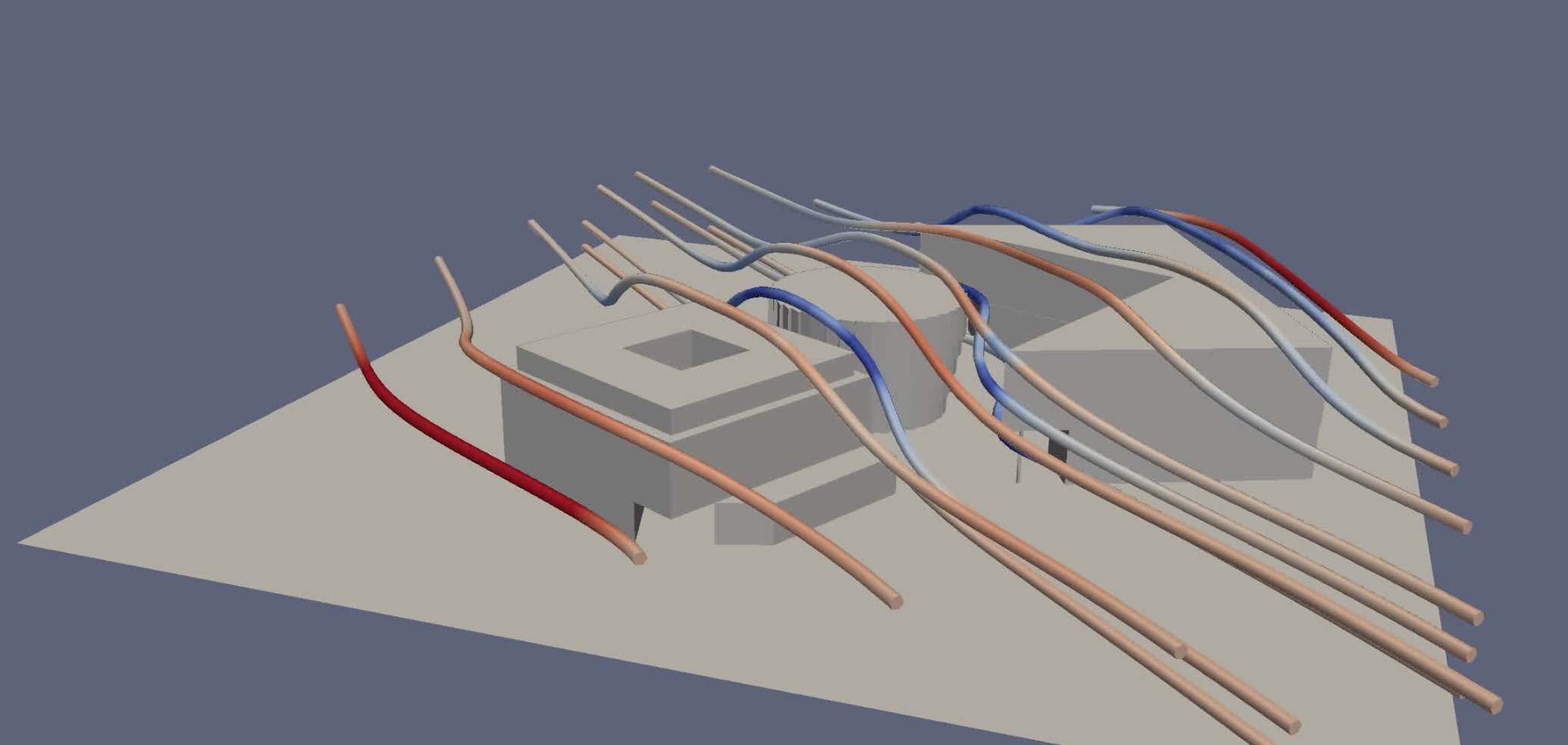
The Stokes solver is a Python class with a solve function. First we initialize a Stokes solver object sso, then we call the solve-function by sso.solve() with supplied problem data defining a Stokes problem. The problem data needed for the Stokes solver is a mesh of the solution domain mesh, and a velocity vector, here [1.0, -1.0, 0], specifying the ambient velocity. The Stokes solver then returns a velocity field velocity_field in the entire solution domain. The velocity field can then be used to compute streamlines for instance. Below streamlines from a Stokes field over a small part of campus Lindholmen are shown in Paraview.

Communication between Unreal Engine and FEniCS-Solvers

Since we use Unreal Engine⁴ for creating a virtual city environment and FEniCS for solving PDE-problems, there’s a need for communication between Unreal and FEniCS. This communication is done with JavaScript Object Notation (JSON⁵) files. Say that we walk around campus Lindholmen in the Unreal environment and are interested in seeing how the air flows around the buildings given a certain wind direction. By choosing Stokes equations as a model for wind flow, noting that we are at Lindholmen, choosing some ambient wind direction, and that we want to visualize the wind flow with streamlines, a JSON-file containing a Python dictionary as the one below should be generated from Unreal Engine and sent to the FEniCS-solver framework.

Note that the Stokes equations are not really suitable for modeling wind flow but are used here to demonstrate the concept of the Unreal-FEniCS-pipeline. We will later incorporate a more advanced flow solver into our pipeline.

If we have named this JSON-file input_stokes.json, it is read as follows by our solver framework:

The Python dictionary in the JSON-file is imported as problem. First an already generated mesh is loaded (or we can also think that we could supply input in the JSON-file to generate a more specific mesh on demand), then the correct model is chosen which solves the defined PDE-problem and returns a solution, here u. The solution is then used to compute the desired output, here streamlines. Finally the output is written to a JSON-file that is sent back to Unreal for visualization.

References