Urban wind simulation
Analysis of wind flow is an important factor in assessing the conditions for pedestrian comfort in a city. The geometries of buildings, in particular tall buildings, and their relative positions have a tremendous effect on the wind experienced by pedestrians on the ground level. Wind is a highly complex phenomenon and the analysis requires the use of sophisticated mathematical modeling and high-performance computing.
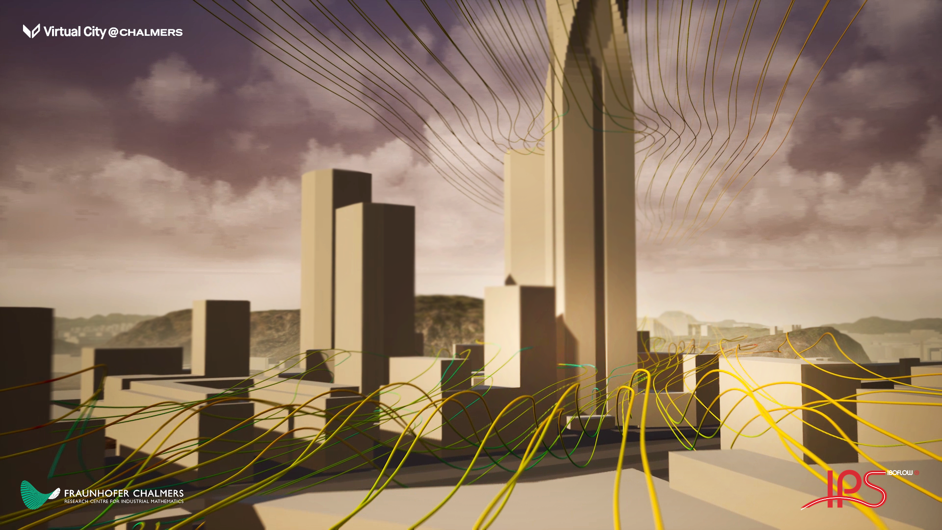
As a first demonstration of the capabilities of the VirtualCity@Chalmers platform, we have analyzed the wind conditions on the Chalmers Lindholmen campus by a Computational Fluid Dynamics (CFD)1 simulation. The simulation is visualized in the film above. The first part of the clip shows a “velocity cut-plane”, which is a visualization of the velocity (magnitude) in a horizontal slice that is visible as a multicolored layer. The plane is taken at a constant height of 15 meters above sea level. Different colors mean different velocity values; bright red means we are near the maximum velocity of approximately 14 meters/second whereas blue colored patches illustrate parts of the domain where the wind velocity is near the minimum of 0 meters/second. Finally, a yellow color indicates that the wind velocity lies somewhere in between the two extremes.
The second part of the clip shows what, in the world of fluid mechanics, is called “streamlines”23 . A streamline is a curve that is tangential to the fluid’s velocity direction. The color of the streamline is determined by the size of the velocity at each point in space. One can imagine the motion of a small element of fluid, usually referred to as a “fluid parcel”, traveling along each streamline.
The software used for the CFD simulation is called IPS IBOFlow4. The tables below summarize the technical information regarding the simulations. The framework used is the newly developed VirtualCity@Chalmers platform5.
Table 1. General information regarding the CFD simulation.| Fluid Solver | IBOFlow, Incompressible Navier-Stokes solver, finite volume |
| Meshing | Fully automatic (only mesh surface as input is required) |
| Boundary treatment | The mirroring immersed boundary method |
| Convective scheme | Ultimate QUICKEST |
| Windspeed | 10 m/s S-SE |
| Turbulence model | K-Omega SST |
| Simulation size | 1.6 km^2 |
| Computational grid | 8 Million cells smallest grid size 50 cm | 50 Million cells smallest grid size 25 cm |
| Computational time breakdown | ||
| Automatic meshing | 30 seconds | 4 minutes |
| CFD Solution | 7 seconds per iteration/time-step | 60 seconds per iteration/time-step |
| Total simulation time | ~ 1 hour | ~12 hours |
All simulations were carried out by the Fraunhofer-Chalmers Research Centre for Industrial Mathematics (FCC)6. Read more about the simulation work behind the video clip above on fcc.chalmers.se/news/ .
The high-performance computer used was an Intel® Xeon Gold 6134 CPU with 196 GB of memory and an NVIDIA Volta V100 graphics card7.